Validation of the Cellocity Software

Validation dataset

In order to validate the underlying analyzers in Cellocity we have generated a “ground truth”, real-world microscopy dataset. The dataset was generated by translating and imaging, with DIC contrast, a fixed monolayer of primary gut epithelium on a high precision linear microscope stage, using a wide selection of magnifications. 10 images were acquired with the stage translated 1 \({\mu m}\) in either the X, Y or both directions simultaneously between frames. Images were acquired on a Nikon Eclipse Ti-2 microscope, equipped with a Photometrics Prime 95B camera (1608x1608, 11 um pixel size). The general structure of the dataset is outlined in the table below.

Objective	Tube lens	Total magnification	Pixel Size (um)	X translation (um)	Y translation (um)	Filename
Nikon 10X/0.45 Air Pln.Apo.Lmbd	1X	10X	1.1235	0	1	fixed_monolayer_DIC_10X_dX-0um_dY-1um_1_MMStack.ome.tif
Nikon 10X/0.45 Air Pln.Apo.Lmbd	1X	10X	1.1235	1	0	fixed_monolayer_DIC_10X_dX-1um_dY-0um_1_MMStack.ome.tif
Nikon 10X/0.45 Air Pln.Apo.Lmbd	1X	10X	1.1235	1	1	fixed_monolayer_DIC_10X_dX-1um_dY-1um_1_MMStack.ome.tif
Nikon 10X/0.45 Air Pln.Apo.Lmbd	1.5X	15X	0.749	0	1	fixed_monolayer_DIC_15X_dX-0um_dY-1um_1_MMStack.ome.tif
Nikon 10X/0.45 Air Pln.Apo.Lmbd	1.5X	15X	0.749	1	0	fixed_monolayer_DIC_15X_dX-1um_dY-0um_1_MMStack.ome.tif
Nikon 10X/0.45 Air Pln.Apo.Lmbd	1.5X	15X	0.749	1	1	fixed_monolayer_DIC_15X_dX-1um_dY-1um_1_MMStack.ome.tif
Nikon 40X/0.6 Air S.Pln.Fl.	1X	40X	0.286	0	1	fixed_monolayer_DIC_40X_dX-0um_dY-1um_1_MMStack.ome.tif
Nikon 40X/0.6 Air S.Pln.Fl.	1X	40X	0.286	1	0	fixed_monolayer_DIC_40X_dX-0um_dY-1um_1_MMStack.ome.tif
Nikon 40X/0.6 Air S.Pln.Fl.	1X	40X	0.286	1	1	fixed_monolayer_DIC_40X_dX-0um_dY-1um_1_MMStack.ome.tif
Nikon 40X/0.6 Air S.Pln.Fl.	1.5X	60X	0.191	0	1	fixed_monolayer_DIC_60Xopt_dX-0um_dY-1um_1_MMStack.ome.tif
Nikon 40X/0.6 Air S.Pln.Fl.	1.5X	60X	0.191	1	0	fixed_monolayer_DIC_60Xopt_dX-1um_dY-0um_1_MMStack.ome.tif
Nikon 40X/0.6 Air S.Pln.Fl.	1.5X	60X	0.191	1	1	fixed_monolayer_DIC_60Xopt_dX-1um_dY-1um_1_MMStack.ome.tif
Nikon 60X/0.7 Air S.Pln.Fl.	1X	60X	0.125	0	1	fixed_monolayer_DIC_60X_dX-0um_dY-1um_1_MMStack.ome.tif
Nikon 60X/0.7 Air S.Pln.Fl.	1X	60X	0.125	1	0	fixed_monolayer_DIC_60X_dX-1um_dY-0um_1_MMStack.ome.tif
Nikon 60X/0.7 Air S.Pln.Fl.	1X	60X	0.125	1	1	fixed_monolayer_DIC_60X_dX-1um_dY-1um_1_MMStack.ome.tif

This dataset allowed us compare the “golden standard” of cell layer dynamics analysis, Particle Image Velocimetry (PIV) analysis, with the less frequently used Optical Flow analysis. Our conclusion mirror what was found in [1], which is that Optical Flow analysis is indeed superior to PIV analysis, both with respect to accuracy and efficiency. The following section will substantiate this finding. All analyses were run on a early 2020 Dell XPS 15 7590 laptop, running Windows 10.

Downloading the validation dataset

The dataset has been deposited into the BioStudies database with the accession number S-BSST461 and can be downloaded from there.

Performing the validation on your local installation

All the validation figures can be re-generated on your local install by running the following code:

from cellocity import validation
from pathlib import Path

inpath = Path("path/to/S-BSST641/")
outpath = Path("path/to/output/folder")

validation.run_base_validation(inpath, outpath)

Alternatively the validation code can be run as a script found in /tests:

After some time you should have generated the 3 figures below in this chapter in your chosen output folder. To test the 5-sgigma analysis run the following code:

from cellocity import validation
from pathlib import Path

inpath = Path("path/to/S-BSST641/")
outpath = Path("path/to/output/folder")

validation.run_5sigma_validation(inpath, outpath)

Alternatively the validation code can be run as a script found in /tests:

First we’ll start by looking at the base validation.

Process time

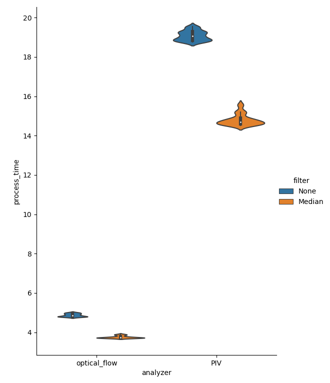
Figure showing violin plots of processing times for individual files in the test dataset. Process time is in seconds and denotes time to run either the OpenPivAnalyzer or the FarenbackAnalyzer on both a Channel and a MedianChannel object created from each file in the dataset. Each file is a 10x1608x1608 16-bit array.

Optical Flow is clearly faster to process all files by a factor of ~3-4X. Now, let’s compare overall accuracy. Since the dataset was created by translating a high precision stage on a well calibrated microscope, we know that the speed of the apparent flow is dependent on the translation distance. In our case we translated the stage 1 \({\mu m}\) between images, and if we set the frame interval to 1 second, then the speed should be 1 \({\mu m/s}\) for the X and Y translation and \(\sqrt{2} = 1.42\) \({\mu m/s}\) for the X+Y translation.

Analysis of flow speeds

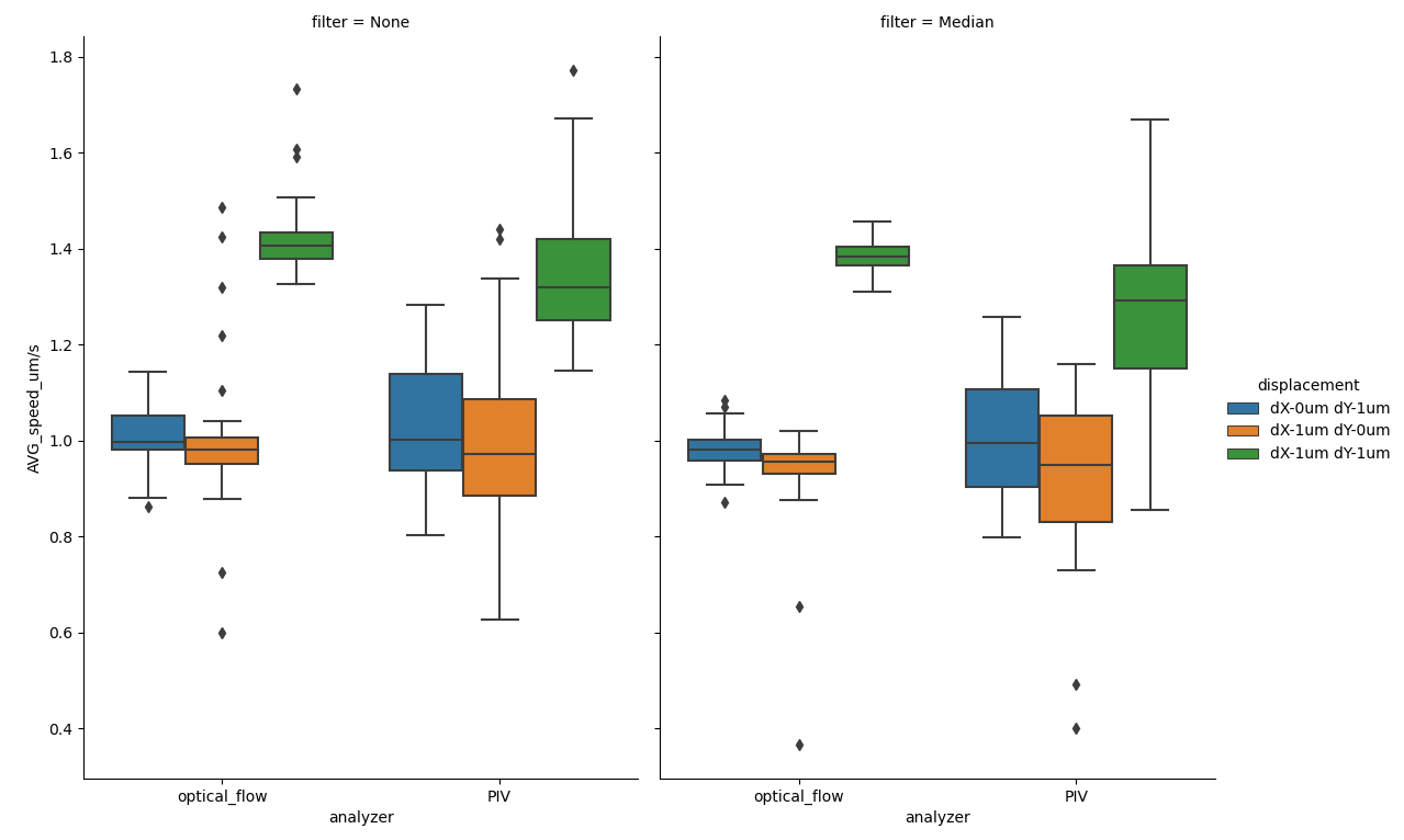
Figure showing box plots of average speeds for each frame for each file in the test dataset. y-axis denotes the speed in \({\mu m/s}\), as read out by the .calculateAverageSpeeds() method of FlowSpeedAnalyser.

Both Analyzers produce results close to the expected, but the OpenPivAnalyzer has a tendency to underestimate the speed and has greater variance.

Cell monolayers grown on loose hydrogel support, as those used in our validation dataset here, are seldom completely planar and portions are often out of focus during imaging. This phenomenon has also been captured in the analysis. If we draw a visualization of the flow generated superimposed on the background Channel, we can study this phenomenon in more detail.

Qualitative vector field comparison

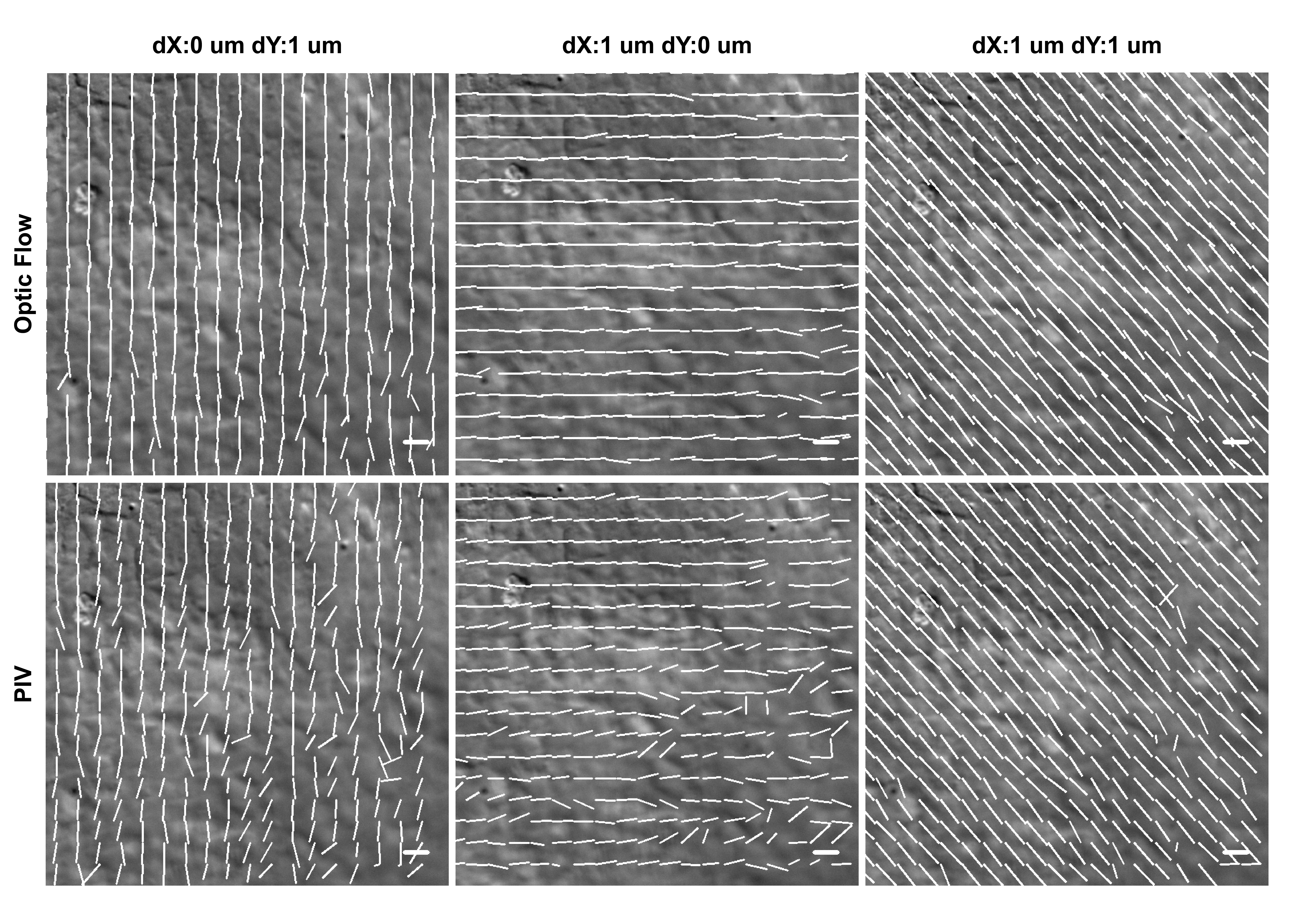
Figure showing flow vector visualization of a 600x600 crop from the bottom right corner of the final frame from the 40X magnification files in the dataset. Images were generated using the .draw_all_flow_frames_superimposed() method common to all FlowAnalysis objects. Horizontal scale bar denotes a flow of 1 \({\mu m/s}\) .

Studying the above figure allows us to get a deeper understanding of why optical flow and PIV differ. Note that the area in the bottom right corner is not properly focused. This causes the PIV algorithm problems in accurately determining the flow, as illustrated by the inhomogeneities in the vector field. This error can be quantified by calculating the alignment index, a measurement on how well each component vector aligns with the average flow. In our test dataset the flow should be close to completely uniform, giving an expected alignment index of 1.0.

Quantitative vector field comparison

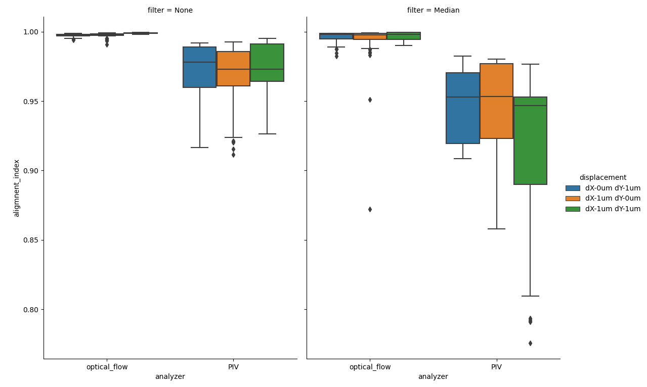
Figure showing box plots of average alignment indexes for each frame for each file in the test dataset. y-axis denotes the Alignment Index (dimensionless), as read out by the .getAvgAlignIdxs() method of AlignmentIndexAnalysis.

Quantifying how well the vector field is aligned allows us to confirm our intital observation that PIV analysis does produce more variability in the direction of the flow vectors. Optical Flow generates alignment indexes very close to the expected value of 1.0, even after temporal median filtering.

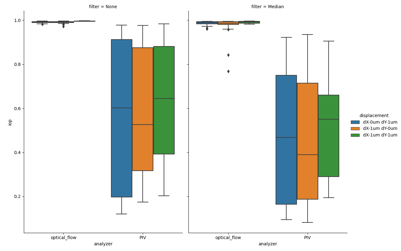
Figure showing box plots of average instantaneous order parameters (iop) for each frame for each file in the test dataset. y-axis denotes the iop (dimensionless), as read out by the .getIops() method of IopAnalysis.

The instantaneous order parameter is a measure of how ordered a vector field is, 0 represents a completely random field and 1 represents a comletely homogenous field, where all vectors have the same direction and magnitude. The expected value for the test data set is 1.

Figure showing flow vector visualization of the diagonal translation at 60X magnification. Images were generated using the .draw_all_flow_frames_superimposed() method common to all FlowAnalysis objects, OpenPivAnalyzer (left) and FarenbackAnalyzer (right). Horizontal scale bar denotes a flow of 1 \({\mu m/s}\) .

Lastly, let’s have a look at the 5-\({\sigma}\) correlation length analysis. 5-\({\sigma}\) correlation length is a way to measure the correlation length in large vector fields. The algorithm finds the average distance at which the direction of velocities are no longer significantly different at a level of 5 standard deviations (\({\sigma}\)). The algorithm was originally presented and utilized in [2]. A more detailed description can be found in the Developer Information.

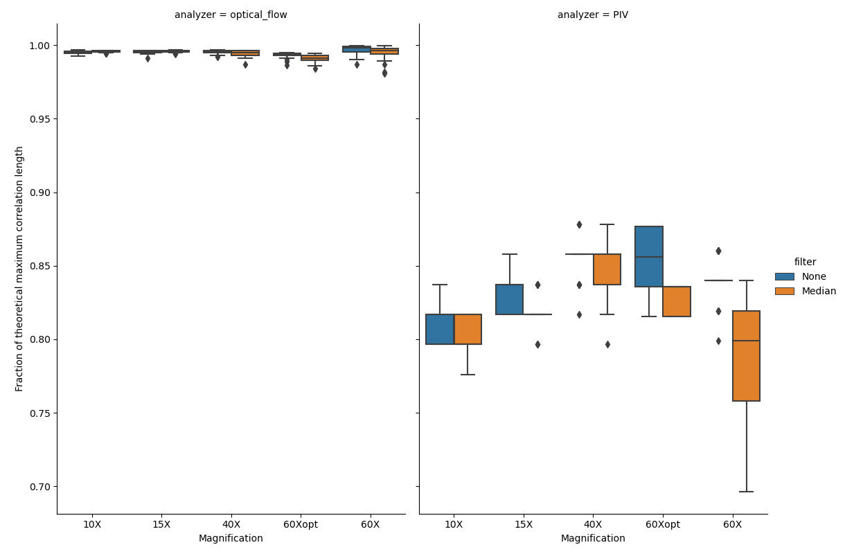
Figure showing box plots of how well the calculated 5-\({\sigma}\) correlation lengths agree with the theoretical maximum value. The value is expressed as a fraction of the calculated correlation length and the theoretical maximum value, which is given by the magnification. Figure generated by passing either OpenPivAnalyzer (right) or FarenbackAnalyzer (left) objects to FiveSigmaAnalysis and calling the calculateCorrelationAllFrames() metod with (orange) and without (blue) temporal median filtering of raw input data.

Once again we see an advantage in utilizing optical flow when compared to PIV. In the figure above the calculated correlation lengths for each file and frame are divided by the size of the field of view (FOV), giving us a metric to compare across magnifications. Optical flow captures almost all of the “true” correlation length, while PIV is only able to capture ~80-85% of the “true” correlation length. Besides being less accurate on this type of data, PIV analysis also downsamples the images, which gives the FiveSigmaAnalysis fewer vectors to use as a basis for correlation length calculations. This is also evident in the average frame processing time (below).

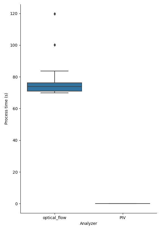
Figure showing a box plot of processing times for individual frames in the test dataset. Process time is in seconds and denotes time to run the FiveSigmaAnalysis on one frame of input data on either FarenbackAnalyzer data (left) or OpenPivAnalyzer data (right).

Here we see an advantage in using PIV because processing times are orders of magnitude lower for the PIV data. The complexity of the 5-\({\sigma}\) correlation length analysis algorithm is \(O(n)\), meaning processing time grows liearly with input size. It is possible to reduce the processing time of optical flow data by tweaking the r_step parameter of the ._get_all_angles() metod of FiveSigmaAnalysis. The default value is 1, which means that the comparison is growing outwards by 1 pixel per step, but a value of 2 would halve the number of comparisons calculated with little expected effect on the final result.

In conclusion

Optical Flow and PIV analysis of transmitted light microscopy time-lapse data is commonly used in studies of confluent cell layer dynamics phenomena, for example collective cell migration and wound healing. This is particularly relevant for studies of primary cells, due to the difficulty in reliably labelling these for cell tracking. To our knowledge, there has not been a systematic evaluation of different pre-processing modalities and optical flow analysis algorithms on actual real-world, non-simulated, microscopy data. We therefore anticipate that others will find this software package and the validation dataset described in this chapter useful.

References

[1]	Dhruv K. Vig, Alex E. Hamby and Charles W. Wolgemuth. On the Quantification of Cellular Velocity Fields. Biophysical Journal, 110:1469-1475, 2016. doi:10.1016/j.bpj.2016.02.032.

[2]

Emma Lång, Anna Połeć, Anna Lång, Marijke Valk, Pernille Blicher, Alexander D. Rowe, Kim A. Tønseth, Catherine J. Jackson, Tor P. Utheim, Liesbeth M. C. Janssen, Jens Eriksson and Stig Ove Bøe. Coordinated collective migration and asymmetric cell division in confluent human keratinocytes without wounding. Nature communications, 1:2041-1723, 2018. doi:10.1038/s41467-018-05578-7.